Lecture IX - Multi-Energy Systems
Energy System Optimization with Julia
Quick Recap from last Week
Energy System Design Problem Overview
Objective: Minimize total annual costs (investment + operational) while respecting budget constraints
Decision Variables:
- Investment variables (First Stage):
- Storage energy capacity (\(e^{nom}_s\))
- Storage charging power (\(p^{ch,nom}_s\))
- Storage discharging power (\(p^{dis,nom}_s\))
- Wind park capacity (\(p^{nom}_w\))
- PV park capacity (\(p^{nom}_v\))
- Operational variables (Second Stage):
- Wind power output (\(p_{w,t,\omega}\))
- PV power output (\(p_{v,t,\omega}\))
- Grid import/export (\(p^{in}_{t,\omega}\), \(p^{out}_{t,\omega}\))
- Storage operation (\(p^{ch}_{s,t,\omega}\), \(p^{dis}_{s,t,\omega}\), \(e_{s,t,\omega}\))
- Investment variables (First Stage):
Key Constraints:
- Investment budget limit
- Power balance
- Component capacity limits
- Storage energy balance
- Storage energy limits
- Storage power limits
The Energy System Design problem combines investment planning (sizing) with operational optimization, enabling comprehensive energy system design. The stochastic formulation considers multiple scenarios to account for uncertainty in renewable generation, demand patterns, and price variations.
Mathematical Formulation
Objective Function
\(\text{Minimize} \quad \sum_{s \in \mathcal{S}} AC^{inv}_s + \sum_{w \in \mathcal{W}} AC^{inv}_w + \sum_{v \in \mathcal{V}} AC^{inv}_v + \sum_{\omega \in \Omega} \pi_{\omega} (AC^{grid,imp}_{\omega} - AR^{grid,exp}_{\omega})\)
Key Constraints
- Investment Budget:
\(\sum_{s \in \mathcal{S}} (C^{E}_s e^{nom}_s + C^{P,ch}_s p^{ch,nom}_s + C^{P,dis}_s p^{dis,nom}_s) + \sum_{w \in \mathcal{W}} C^{W}_w p^{nom}_w + \sum_{v \in \mathcal{V}} C^{PV}_v p^{nom}_v \leq B^{max}\)
- Power Balance:
\(\sum_{w \in \mathcal{W}} p_{w,t,\omega} + \sum_{v \in \mathcal{V}} p_{v,t,\omega} + (p^{in}_{t,\omega} - p^{out}_{t,\omega}) + \sum_{s \in \mathcal{S}} (p^{dis}_{s,t,\omega} - p^{ch}_{s,t,\omega}) = d_{t,\omega} \quad \forall t \in \mathcal{T}, \omega \in \Omega\)
- Component Capacity Limits:
\(0 \leq p_{w,t,\omega} \leq f_{w,t,\omega} p^{nom}_w \quad \forall w \in \mathcal{W}, t \in \mathcal{T}, \omega \in \Omega\) \(0 \leq p_{v,t,\omega} \leq f_{v,t,\omega} p^{nom}_v \quad \forall v \in \mathcal{V}, t \in \mathcal{T}, \omega \in \Omega\) \(0 \leq p^{ch}_{s,t,\omega} \leq p^{ch,nom}_s \quad \forall s \in \mathcal{S}, t \in \mathcal{T}, \omega \in \Omega\) \(0 \leq p^{dis}_{s,t,\omega} \leq p^{dis,nom}_s \quad \forall s \in \mathcal{S}, t \in \mathcal{T}, \omega \in \Omega\) \(DoD_s e^{nom}_s \leq e_{s,t,\omega} \leq e^{nom}_s \quad \forall s \in \mathcal{S}, t \in \mathcal{T}, \omega \in \Omega\)
- Storage Energy Balance:
\(e_{s,t,\omega} = (1-sdr_s)e_{s,t-1,\omega} + \eta^{ch}_s p^{ch}_{s,t,\omega} - \frac{p^{dis}_{s,t,\omega}}{\eta^{dis}_s} \quad \forall s \in \mathcal{S}, t \in \mathcal{T}, \omega \in \Omega\)
Model Characteristics
- Two-stage stochastic Linear Programming (LP) problem
- Combines investment and operational decisions
- Large-scale optimization problem
- Requires efficient solution methods
- Considers multiple scenarios for robust decision-making
The model can be adapted to specific use cases, i.e., if a wind park already has a fixed capacity, the corresponding variable can be converted to a parameter. The stochastic formulation allows for more robust investment decisions by considering multiple scenarios.
Additional Constraints
The basic model can be extended with various constraints, partly covered from previous lectures:
Generator Constraints
- Minimum up/down times
- Start-up and shut-down costs
- Ramp rate limits
- Minimum load constraints
- Part-load efficiency curves
Storage Constraints
- Ramp rate limits for charging/discharging
- Mutual exclusion constraints
- Cycle limits (daily/weekly/seasonal)
- State of charge dependent efficiency
- Temperature dependent operation
- Degradation effects
- Multiple storage technologies with different characteristics
Grid Connection
- Maximum import/export power limits
- Grid fees and tariffs
- Ancillary service requirements
Renewable Generation
- Curtailment limits
System-wide Constraints
- Reserve requirements
- Island operation capability
- Multiple energy carriers
- Environmental constraints
- Regulatory requirements
These additional constraints can be included based on the specific requirements of the energy system being designed. Each constraint adds complexity but may be necessary for realistic modeling.
Implementation Insights
- Data structures use NamedTuples for efficient parameter storage
- Results are stored in DataFrames for easy analysis
- Key metrics tracked:
- Total system cost
- Investment costs by component
- Operational costs
- Component capacities
- Storage operation
- Grid interaction
- Sensitivity analysis capabilities:
- Budget variations
- Electricity price changes
- Component cost variations
The tutorial demonstrated how to implement and solve the stochastic design problem using Julia and JuMP, including comprehensive sensitivity analysis of key parameters such as investment budget and electricity prices.
Solutions from last Week
- The tutorials from last week will again be available on Friday
- You can access them in the project folder on Github
- Click on the little cat icon on the bottom right
. . .
You can ask questions anytime in class or via email!
Excursion: Two-Stage Stochastic Programming
Problem Structure vs. Solution Method
A two-stage stochastic programming problem is characterized by its decision structure, not its solution method. The key aspects are:
- Decision Stages:
- First stage (here-and-now): Decisions made before uncertainty is revealed
- Second stage (wait-and-see): Decisions made after uncertainty is revealed
- Information Structure:
- First stage: Decisions based on known parameters and probability distributions
- Second stage: Decisions based on observed scenario realizations
The “two-stage” classification refers to the logical structure and timing of decisions, not how the problem is solved computationally.
Solution Approaches
Monolithic Approach
- Solve the entire problem as one large optimization model
- All constraints and variables are included in a single mathematical program
- Advantages:
- Simpler implementation
- Direct solution using standard solvers
- No need for specialized algorithms
- Disadvantages:
- Can become computationally challenging for large problems
- May require significant memory resources
Decomposition Methods
- Break the problem into smaller subproblems
- Examples:
- Benders decomposition: Iteratively solves a master problem (first stage) and subproblems (second stage) by adding cuts that approximate the second-stage cost
- Progressive hedging: Solves each scenario independently and iteratively adjusts solutions to achieve consensus across scenarios
- L-shaped method: Similar to Benders, but specifically designed for two-stage stochastic linear programs with a special structure
- Advantages:
- Can handle larger problems
- More efficient for certain problem structures
- Disadvantages:
- More complex implementation
- May require specialized algorithms
Energy System Design Example
In our energy system design problem:
First Stage (Investment)
- Storage capacity decisions
- Wind park capacity
- PV park capacity
- Made before knowing:
- Renewable generation profiles
- Demand patterns
- Electricity prices
Second Stage (Operation)
- Power dispatch decisions
- Storage operation
- Grid interaction
- Made after observing:
- Actual renewable generation
- Real demand
- Current market prices
Whether we solve this as one large optimization problem or use decomposition methods, it remains a two-stage stochastic program due to its decision structure and information flow.
Mathematical Representation
The general form of a two-stage stochastic program is:
\(\min_{x} \quad c^T x + \mathbb{E}_{\omega}[Q(x,\omega)]\)
where:
- \(x\) represents first-stage decisions
- \(Q(x,\omega)\) represents the second-stage problem for scenario \(\omega\)
- \(\mathbb{E}_{\omega}\) denotes the expectation over all scenarios
This structure can be solved:
- As one large optimization problem (monolithic)
- Using decomposition methods
- Through other specialized algorithms
The choice of solution method depends on:
- Problem size
- Available computational resources
- Required solution time
- Implementation complexity
The two-stage structure provides a framework for modeling decision-making under uncertainty, regardless of the computational approach used to solve it.
Introduction to Multi-Energy Systems
Multi-Energy Systems: Definition
A multi-energy system is a system that combines multiple energy carriers (e.g. electricity, hydrogen, heat, etc.) to meet the energy demand of a specific application.
Multi-Energy Systems: Example Hydrogen Value Chain
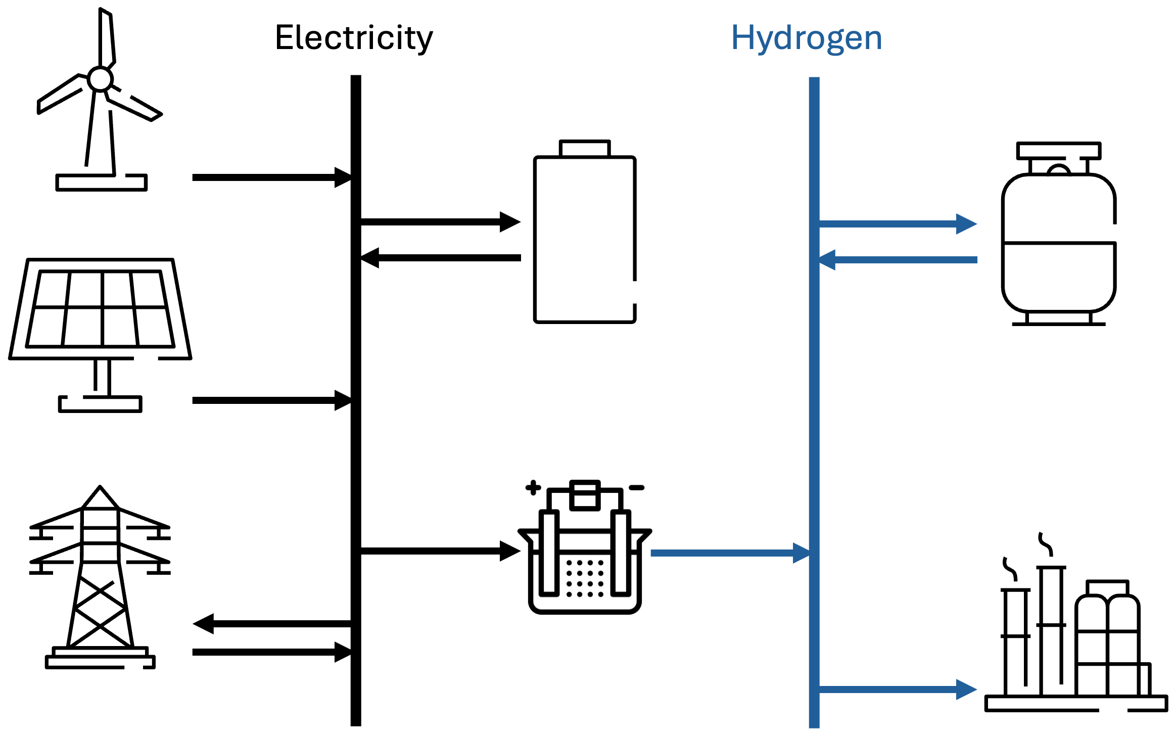
The figure shows a multi-energy system with:
- Renewable energy sources (PV and Wind) and grid connection
- Electric bus bar for power distribution
- Electrolyzer for hydrogen production
- Hydrogen bus bar for hydrogen distribution
- Hydrogen storage
- Hydrogen demand
Multi-Energy System Design Problem
In this lecture, we extend the Stochastic System Design problem to include investment decisions for multi-energy systems. This allows us to:
- Optimize technology selection over the entire energy value chain
- Determine optimal component sizes
- Balance investment and operational costs
- Plan local multi-energy systems holistically (e.g. electricity, hydrogen, heat, etc.)
Remember: The design problem combines investment planning (sizing) with operational optimization, enabling comprehensive (multi-)energy system design.
Key Components
We will focus on optimizing:
- Storage systems for electricity and hydrogen
- Wind parks
- PV parks
- Electrolyzers
- Electric market participation
… while fullfilling a fixed hydrogen demand. Additionally, we consider a maximum investment budget.
All nominal sizes will be decision variables in our optimization model.
Mathematical Formulation of the Stochastic Design Problem for Multi-Energy Systems
… on the simple example of the hydrogen value chain with electricity and hydrogen as mediums
Sets
- \(\mathcal{T}\) - Set of time periods indexed by \(t \in \{1,2,...,|\mathcal{T}|\}\)
- \(\mathcal{S}\) - Set of storage systems indexed by \(s \in \{1,2,...,|\mathcal{S}|\}\)
- \(\mathcal{S}_{\text{El}}\) - Subset of \(\mathcal{S}\) of electricity storage systems
- \(\mathcal{S}_{\text{H2}}\) - Subset of \(\mathcal{S}\) of hydrogen storage systems
- \(\mathcal{W}\) - Set of wind parks indexed by \(w \in \{1,2,...,|\mathcal{W}|\}\)
- \(\mathcal{V}\) - Set of PV parks indexed by \(v \in \{1,2,...,|\mathcal{V}|\}\)
- \(\mathcal{X}\) - Set of electrolyzers indexed by \(x \in \{1,2,...,|\mathcal{X}|\}\)
- \(\Omega\) - Set of scenarios indexed by \(\omega \in \{1,2,...,|\Omega|\}\)
New additions to the sets:
- \(\mathcal{S}_{\text{El}}\) and \(\mathcal{S}_{\text{H2}}\) to distinguish between electricity and hydrogen storage
- \(\mathcal{X}\) for electrolyzers as a new component type
Decision Variables
Investment Variables (First Stage)
- \(e^{nom}_s\) - Nominal energy capacity of storage \(s\) [MWh]
- \(p^{ch,nom}_s\) - Nominal charging power of storage \(s\) [MW]
- \(p^{dis,nom}_s\) - Nominal discharging power of storage \(s\) [MW]
- \(p^{nom}_w\) - Nominal power of wind park \(w\) [MW]
- \(p^{nom}_v\) - Nominal power of PV park \(v\) [MW]
- \(p^{nom}_x\) - Nominal power of electrolyzer \(x\) [MW]
Operational Variables (Second Stage)
- \(p_{w,t,\omega}\) - Power output of wind park \(w\) at time \(t\) in scenario \(\omega\) [MW]
- \(p_{v,t,\omega}\) - Power output of PV park \(v\) at time \(t\) in scenario \(\omega\) [MW]
- \(p^{in}_{t,\omega}\) - Power inflow through market at time \(t\) in scenario \(\omega\) [MW]
- \(p^{out}_{t,\omega}\) - Power outflow through market at time \(t\) in scenario \(\omega\) [MW]
- \(p^{ch}_{s,t,\omega}\) - Charging power of storage \(s\) at time \(t\) in scenario \(\omega\) [MW]
- \(p^{dis}_{s,t,\omega}\) - Discharging power of storage \(s\) at time \(t\) in scenario \(\omega\) [MW]
- \(e_{s,t,\omega}\) - Energy level of storage \(s\) at time \(t\) in scenario \(\omega\) [MWh]
- \(p_{x,t,\omega}\) - Power consumption of electrolyzer \(x\) at time \(t\) in scenario \(\omega\) [MW]
- \(h_{x,t,\omega}\) - Hydrogen production of electrolyzer \(x\) at time \(t\) in scenario \(\omega\) [MW]
New operational variables for the electrolyzer:
- \(p_{x,t,\omega}\) for power consumption
- \(h_{x,t,\omega}\) for hydrogen production
Annual Cost Variables
- \(AC^{inv}_s\) - Annual investment cost for storage \(s\) [EUR/year]
- \(AC^{inv}_w\) - Annual investment cost for wind park \(w\) [EUR/year]
- \(AC^{inv}_v\) - Annual investment cost for PV park \(v\) [EUR/year]
- \(AC^{inv}_x\) - Annual investment cost for electrolyzer \(x\) [EUR/year]
- \(AC^{grid,imp}_{\omega}\) - Annual grid electricity import cost in scenario \(\omega\) [EUR/year]
- \(AR^{grid,exp}_{\omega}\) - Annual grid electricity export revenue in scenario \(\omega\) [EUR/year]
New cost variable: \(AC^{inv}_x\) for electrolyzer investment costs
Parameters
Investment Costs (First Stage)
- \(C^{E}_s\) - Cost per MWh of energy capacity for storage \(s\) [EUR/MWh]
- \(C^{P,ch}_s\) - Cost per MW of charging power capacity for storage \(s\) [EUR/MW]
- \(C^{P,dis}_s\) - Cost per MW of discharging power capacity for storage \(s\) [EUR/MW]
- \(C^{W}_w\) - Cost per MW of wind park \(w\) [EUR/MW]
- \(C^{PV}_v\) - Cost per MW of PV park \(v\) [EUR/MW]
- \(C^{X}_x\) - Cost per MW of electrolyzer \(x\) [EUR/MW]
- \(F^{PVAF}\) - Present value annuity factor for investment costs
- \(B^{max}\) - Maximum investment budget [EUR]
New investment cost parameter: \(C^{X}_x\) for electrolyzer capacity costs
Operational Parameters (Second Stage)
- \(\eta^{ch}_s\) - Charging efficiency of storage \(s\)
- \(\eta^{dis}_s\) - Discharging efficiency of storage \(s\)
- \(sdr_s\) - Self-discharge rate of storage \(s\) per time step
- \(DoD_s\) - Depth of discharge limit for storage \(s\) [%]
- \(f_{w,t,\omega}\) - Wind capacity factor at time \(t\) in scenario \(\omega\) for wind park \(w\)
- \(f_{v,t,\omega}\) - Solar capacity factor at time \(t\) in scenario \(\omega\) for PV park \(v\)
- \(d_{t,\omega}\) - Hydrogen demand at time \(t\) in scenario \(\omega\) [MW]
- \(c^{MP}_{t,\omega}\) - Grid electricity market price at time \(t\) in scenario \(\omega\) [EUR/MWh]
- \(c^{TaL}\) - Grid electricity taxes and levies (including Netzentgelt) [EUR/MWh]
- \(\beta_x\) - Conversion factor of electrolyzer \(x\) [MW H2/MW El]
- \(\pi_{\omega}\) - Probability of scenario \(\omega\)
Changes in operational parameters:
- \(d_{t,\omega}\) now represents hydrogen demand instead of electricity demand
- New parameter \(\beta_x\) for electrolyzer conversion efficiency
Objective Function
\(\text{Minimize} \quad \sum_{s \in \mathcal{S}} AC^{inv}_s + \sum_{w \in \mathcal{W}} AC^{inv}_w + \sum_{v \in \mathcal{V}} AC^{inv}_v + \sum_{x \in \mathcal{X}} AC^{inv}_x + \sum_{\omega \in \Omega} \pi_{\omega} (AC^{grid,imp}_{\omega} - AR^{grid,exp}_{\omega})\)
Changes in objective function: Added electrolyzer investment costs \(\sum_{x \in \mathcal{X}} AC^{inv}_x\)
Annual Cost Constraints
Investment Costs (First Stage)
\(AC^{inv}_s = \frac{C^{E}_s}{F^{PVAF}} e^{nom}_s + C^{P,ch}_s p^{ch,nom}_s + C^{P,dis}_s p^{dis,nom}_s \quad \forall s \in \mathcal{S}\) \(AC^{inv}_w = \frac{C^{W}_w}{F^{PVAF}} p^{nom}_w \quad \forall w \in \mathcal{W}\) \(AC^{inv}_v = \frac{C^{PV}_v}{F^{PVAF}} p^{nom}_v \quad \forall v \in \mathcal{V}\) \(AC^{inv}_x = \frac{C^{X}_x}{F^{PVAF}} p^{nom}_x \quad \forall x \in \mathcal{X}\)
Investment Budget
\(\sum_{s \in \mathcal{S}} (C^{E}_s e^{nom}_s + C^{P,ch}_s p^{ch,nom}_s + C^{P,dis}_s p^{dis,nom}_s) + \sum_{w \in \mathcal{W}} C^{W}_w p^{nom}_w + \sum_{v \in \mathcal{V}} C^{PV}_v p^{nom}_v + \sum_{x \in \mathcal{X}} C^{X}_x p^{nom}_x \leq B^{max}\)
Changes in investment budget: Added electrolyzer investment costs \(\sum_{x \in \mathcal{X}} C^{X}_x p^{nom}_x\)
Grid Electricity Costs (Second Stage)
\(AC^{grid,imp}_{\omega} = \sum_{t \in \mathcal{T}} (c^{MP}_{t,\omega} + c^{TaL}) p^{in}_{t,\omega} \quad \forall \omega \in \Omega\) \(AR^{grid,exp}_{\omega} = \sum_{t \in \mathcal{T}} c^{MP}_{t,\omega} p^{out}_{t,\omega} \quad \forall \omega \in \Omega\)
Constraints
Power Balance (Electricity)
\(\sum_{w \in \mathcal{W}} p_{w,t,\omega} + \sum_{v \in \mathcal{V}} p_{v,t,\omega} + (p^{in}_{t,\omega} - p^{out}_{t,\omega}) + \sum_{s \in \mathcal{S}_{\text{El}}} (p^{dis}_{s,t,\omega} - p^{ch}_{s,t,\omega}) = \sum_{x \in \mathcal{X}} p_{x,t,\omega} \quad \forall t \in \mathcal{T}, \omega \in \Omega\)
Changes in electricity balance:
- Uses \(\mathcal{S}_{\text{El}}\) subset for electricity storage
- Right-hand side changed from demand to electrolyzer consumption
Hydrogen Balance
\(\sum_{x \in \mathcal{X}} h_{x,t,\omega} + \sum_{s \in \mathcal{S}_{\text{H2}}} (p^{dis}_{s,t,\omega} - p^{ch}_{s,t,\omega}) = d_{t,\omega} \quad \forall t \in \mathcal{T}, \omega \in \Omega\)
New constraint:
Hydrogen balance equation considering:
- Hydrogen production from electrolyzers
- Hydrogen storage operations
- Hydrogen demand
Component Limits
Wind Parks
\(0 \leq p_{w,t,\omega} \leq f_{w,t,\omega} p^{nom}_w \quad \forall w \in \mathcal{W}, t \in \mathcal{T}, \omega \in \Omega\)
PV Parks
\(0 \leq p_{v,t,\omega} \leq f_{v,t,\omega} p^{nom}_v \quad \forall v \in \mathcal{V}, t \in \mathcal{T}, \omega \in \Omega\)
Storage Systems
\(0 \leq p^{ch}_{s,t,\omega} \leq p^{ch,nom}_s \quad \forall s \in \mathcal{S}, t \in \mathcal{T}, \omega \in \Omega\) \(0 \leq p^{dis}_{s,t,\omega} \leq p^{dis,nom}_s \quad \forall s \in \mathcal{S}, t \in \mathcal{T}, \omega \in \Omega\) \(DoD_s e^{nom}_s \leq e_{s,t,\omega} \leq e^{nom}_s \quad \forall s \in \mathcal{S}, t \in \mathcal{T}, \omega \in \Omega\)
Storage Energy Balance
\(e_{s,t,\omega} = (1-sdr_s)e_{s,t-1,\omega} + \eta^{ch}_s p^{ch}_{s,t,\omega} - \frac{p^{dis}_{s,t,\omega}}{\eta^{dis}_s} \quad \forall s \in \mathcal{S}, t \in \mathcal{T}, \omega \in \Omega\)
Electrolyzer Constraints
\(0 \leq p_{x,t,\omega} \leq p^{nom}_x \quad \forall x \in \mathcal{X}, t \in \mathcal{T}, \omega \in \Omega\) \(h_{x,t,\omega} = \beta_x p_{x,t,\omega} \quad \forall x \in \mathcal{X}, t \in \mathcal{T}, \omega \in \Omega\)
New constraints for electrolyzer:
- Power consumption limits
- Conversion relationship between power consumption and hydrogen production
Literature Review: Multi-Energy Systems and Energy Hubs
Conceptual Foundation
Multi-energy systems (MES) and energy hubs represent a fundamental shift in energy system design, moving from single-carrier optimization to integrated multi-carrier approaches. The energy hub concept was originally introduced by Geidl and Andersson (2007) as a framework for optimal coupling of energy infrastructures, enabling the integration of electricity, heat, gas, and other energy carriers within a unified optimization framework.
The energy hub concept provides a systematic approach to model and optimize multi-carrier energy systems, enabling the integration of renewable energy sources, storage technologies, and energy conversion processes.
Recent Literature Reviews
Several comprehensive literature reviews have been conducted in recent years, highlighting the growing importance of multi-energy systems:
Uncertainty Modeling and Optimization
Recent reviews by Jasinski et al. (2023), Lasemi et al. (2022), and Onen, Mokryani, and Zubo (2022) focus on uncertainty modeling approaches in energy hub optimization. These reviews identify three main approaches: - Stochastic Programming: Using scenario-based optimization with Monte Carlo simulation - Robust Optimization: Providing conservative but computationally efficient solutions - Hybrid Methods: Combining the advantages of both approaches
Comprehensive Framework Reviews
Papadimitriou et al. (2023) provides a systematic review of modeling formulations, optimization methods, and market interactions in energy hubs. Ding et al. (2022) extends this analysis to include trading and control structures for handling large-scale datasets.
Historical Development
Earlier reviews by Maroufmashat et al. (2019) and Son et al. (2021) identified the hydrogen economy as a major application area for energy hubs, following the original proposals by Geidl and Andersson (2007). These reviews systematically analyzed 200+ articles published between 2007-2017, establishing the foundation for current research directions.
Key Research Directions
Hydrogen and Power-to-X Integration
Recent literature identifies hydrogen and Power-to-X (P2X) technologies as critical future research directions. Kountouris et al. (2023) developed an optimization model for P2X-integrated energy hubs applied to an industrial park in Denmark, demonstrating the economic viability of hydrogen, methanol, and ammonia production.
Industrial Applications
Wassermann et al. (2022) addressed the planning and operation problem for hydrogen demand in refinery applications, presenting MILP model extensions for water electrolysis and cavern storage. This work demonstrates the practical application of energy hub concepts to real-world industrial decarbonization projects.
Uncertainty and Computational Challenges
The representation of renewable energy uncertainty is identified as a core challenge across multiple reviews. Ringkjöb, Haugan, and Solbrekke (2018), who reviewed 75 energy system modeling frameworks, conclude that high spatiotemporal resolution is essential for accurate RES representation, but comes at significant computational cost.
The trade-off between model fidelity and computational burden is a central challenge in multi-energy system optimization, particularly when considering renewable energy uncertainty.
Solution Methods and Frameworks
Decomposition Approaches
Several studies demonstrate the effectiveness of Benders decomposition for energy hub optimization. Mansouri et al. (2020), Chen et al. (2019), and Hemmati, Ghaderi, and Ghazizadeh (2018) use Benders decomposition to separate dimensioning decisions (master problem) from operational optimization (subproblems), enabling efficient solution of large-scale problems.
Advanced Modeling Frameworks
Recent frameworks address computational complexity through innovative approaches:
- SpineOpt (Ihlemann et al. (2022)): A flexible Julia-based framework allowing variable temporal resolution per system component
- AnyMod (Göke (2021)): A pure linear model formulation designed for macro-energy system planning with full-year time series
- ficus (Atabay (2017)): An industrial energy system optimization framework based on the urbs framework (Dorfner (2016))
Temporal Resolution Challenges
Gonzato, Bruninx, and Delarue (2021) analyzed techniques for reducing temporal scope in expansion planning models with long-term storage, recommending against temporal reductions and advocating for full-year time series inclusion to prevent biases in system design.
Hydrogen Supply Chain Integration
The integration of hydrogen supply chain network design (HSCND) with energy hub optimization represents an emerging research area. Li, Manier, and Manier (2019) provides a comprehensive review of HSCND optimization approaches, while Riera, Lima, and Knio (2023) reviews hydrogen production and supply chain modeling specifically.
The integration of hydrogen supply chain optimization with energy hub concepts enables comprehensive planning of green hydrogen value chains from production to end-use applications.
Open Source Tools and Frameworks
Several reviews assess the maturity and capabilities of open-source energy system optimization tools:
- Groissböck (2019) evaluates the maturity of open-source tools for serious applications
- Oberle and Elsland (2019) assesses the ability of open-access models to evaluate current energy scenarios
- Pfenninger, Hawkes, and Keirstead (2014) provides a broader perspective on energy systems modeling challenges
Future Research Directions
Recent literature reviews identify several critical future research directions:
- Technology Integration: Further development of hydrogen, P2X, and CCUS technologies in integrated energy hubs
- Real-world Applications: Development of practical applications and business cases for energy hub concepts
- Computational Efficiency: Development of efficient modeling schemes and solution algorithms for uncertainty representation
- Industrial Decarbonization: Application of energy hub concepts to hard-to-abate industrial sectors
The energy hub concept has evolved from a theoretical framework to a practical tool for industrial decarbonization, with growing applications in hydrogen value chains and Power-to-X systems.
Literature II
Literature
Literature I
For more interesting literature to learn more about Julia, take a look at the literature list of this course.